 Download brochure
Room Correction
Introduction
Today there are a number of room correction solutions available on the market. They all more or less operate in similar fashion in fundamental ways.
All systems use ordinary time gated measurements that all shares the same fundamental problem; a single measurement doesn’t correlate very well with how sound in a room is perceived by a listener. This is a well-known fact that all loudspeaker designers are aware of but nevertheless these are the measurement tools that are presently obtainable.
The first room correction product became available about 20 years ago. It relied on measuring the speaker response at a single listening position. The measurement didn’t correlate well with human perception of sound but it managed to improve the sound to some extent in some however not all cases and there were obvious problems.
In an attempt to solve the measurement problem there was a migration towards using additional measuring positions. New systems became available that measured the response in two or more locations in the room and they improved the room correction to some degree compared to the earliest system. The systems using multiple measuring positions are capturing something that approaches the power response from the loudspeaker in the room. They often put different emphasis on the different measuring positions and they don’t use enough positions so it is not entirely scientifically accurate to claim they capture the power response but since it is commonly stated we will hence forth simplify matters and refer to these systems as power response based correction systems.
The power response based correction systems are however lacking vital time domain information because once you move from measuring in a single listening position to several the time domain information is unavoidably lost. They started with a measurement that didn’t correlate well to human perception of sound to begin with, by measuring in several locations they have improved the measurement but in the process lost the time domain information. Now what’s left to operate on is the frequency domain information, i.e. the frequency response.
The correction algorithms use the measured frequency response information and simply invert the measured frequency deviations and use it as a pre-emphasis on the music signal about to be played back. The time domain is obtained assuming that the measured response deviations are all minimum phase, which they are not, through a simple Hilbert transform. There is usually a little bit more intelligence needed in the process though. As an example it is not possible to boost huge dips at lower frequencies, it would cause severe distortion, clipping and overheating. Let’s say we have a small loudspeaker with a 6.5” base driver. If we have a room induced dip of 8 dB at 75 Hz it is not possible to boost that frequency by 8 dB because the driver would not be able to physically move enough air to generate a sufficient amount of sound pressure at 75 Hz. It could also possibly cause amplifier clipping or at the very least produce significant distortion from the driver that’s trying to perform outside of its capability. Most systems avoid these kinds of pitfalls.
This more or less describes the current state of art in room correction systems. There are flaws caused by predominantly measurement limitations and some people like the results but some don’t. The corrections are sometimes improving the sound and sometimes not so much even possibly making things worse. There is also a lack of uniformity of the sound in the room; the base might be good in one location but booming and unarticulated in another. Some people also claim that the room correction systems sound artificial to some degree.
It seems there is a need for a completely new approach and that would require a new measurement method and new correction algorithms that don’t just invert the measured frequency response with some add on rules ignoring the time domain.
The Böhmer Audio Room Compensation System is the first of the second generation of room correction systems incorporating a groundbreaking new measurement method and fundamentally different correction algorithms to solve the primary weaknesses universally exhibited by earlier room correction systems.
How to carry out measurements
Regular methods for measuring loudspeaker responses in listening rooms usually use one or more omnidirectional measurement microphones in one or several locations in the room. They usually capture a mix of sound pressure at the listening position or positions and a number of other positions in the room together forming a composite measurement exhibiting something that approaches the power response in the room. A power response measurement does not inherently contain any time domain information and is not a very useful basis for room correction as we will see later.
The Böhmer Audio Room Compensation uses a unique psychoacoustically based measurement method that is entirely different from above. The method is capable of capturing the essential time domain information together with the more common frequency domain information. The key being that the method captures the measurement in both time and frequency similarly to our hearing. The method, in a few words, uses one measurement position in front of the loudspeaker and captures the response from the speaker by applying a complex time gating method that gates the measured signal from the loudspeaker in a fashion that correlates to how the sound is perceived by a listener.
Resonances within a room are time domain phenomena
To visualize the resonant behavior in a room we have built a computer model of a typical well behaved listening room fitted with various absorbers and diffusers in an attempt to optimize it for music playback. The room is about 6 m / 20 feet long, 4.5 m / 15 feet wide and has a 2.7m / 9 feet ceiling. Reverberation time in the room is very well controlled around 0.4 s (+/-0.1 s) across the entire frequency spectra with reverberation time becoming longer only at the lowest frequencies below 65 Hz. The early reflection surfaces in the room have all been treated with a combination of diffusion and absorption and there are four low frequency membrane absorbers in the corners of the room, often referred to as tube traps. We think it is fair to say that the room is as optimal as any typical listening room will be without resorting to other measures of treatment than add on absorbers and diffusers.
Below is a 3D computer generated image of a view from the left back corner of the room followed by a 2D top view.
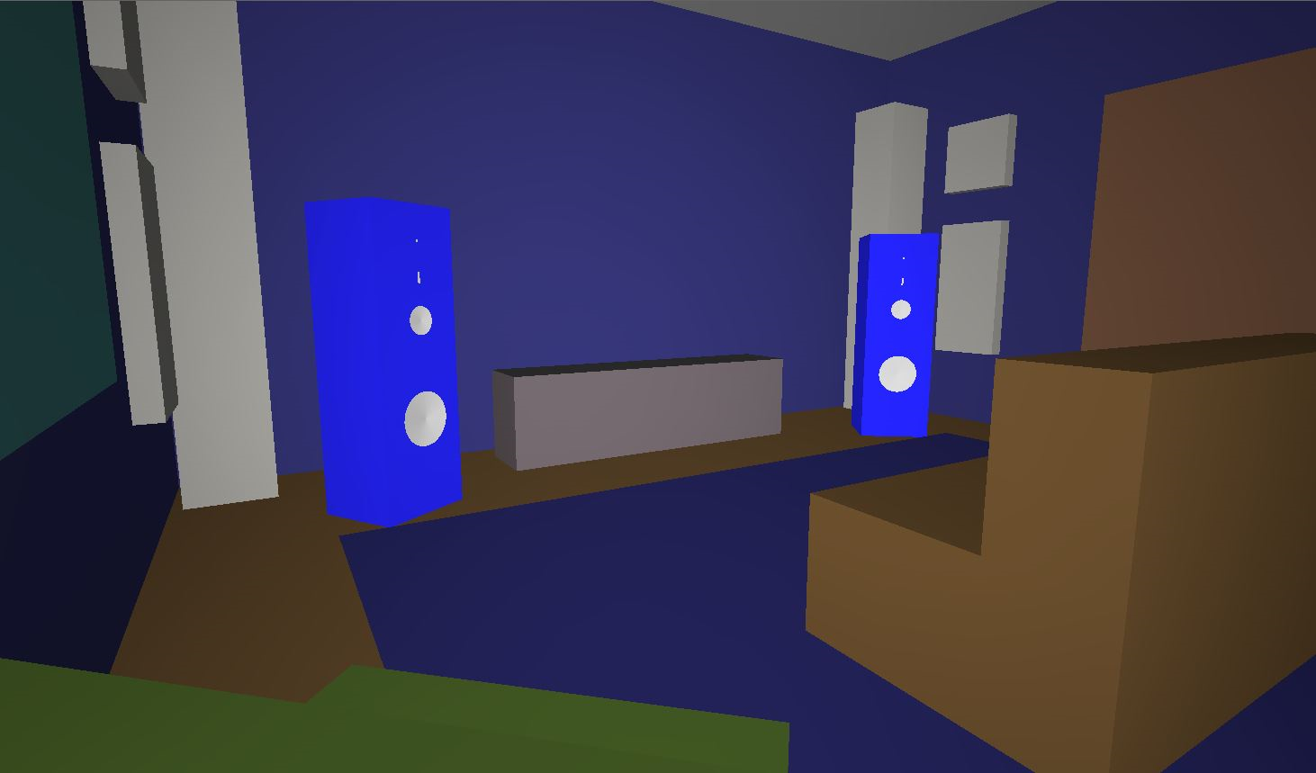 Fig 3.1: A 3D view from the simulated room
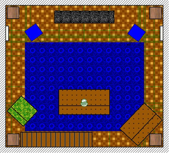
Fig 3.2: 2D drawing of the simulated room
The steady state resonance sound field in the room is the only thing that is captured by a power response measurement. Below is a series of images of the steady state resonant sound field in the room at different frequencies. The two blue circles in the images are the loudspeakers and the yellow circle is at the listening position. The sound level is color coded; a darker color signifies a lower sound pressure level and a brighter more reddish a higher. The color bar shows how the sound pressure levels correspond to the different colors.

Fig 3.3: Sound pressure color bar
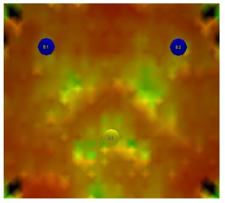
Fig 3.4: Steady state sound field at 74 Hz in the simulated room
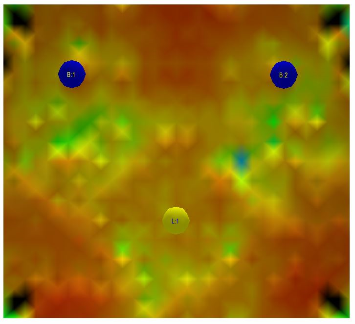
Fig 3.5: Steady state sound field at 80 Hz in the simulated room
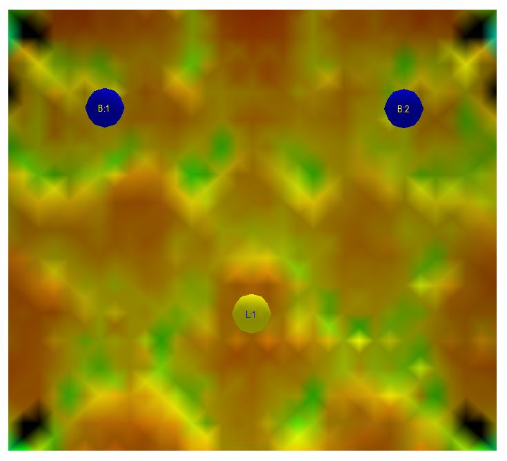
Fig 3.6: Steady state sound field at 160 Hz in the simulated room
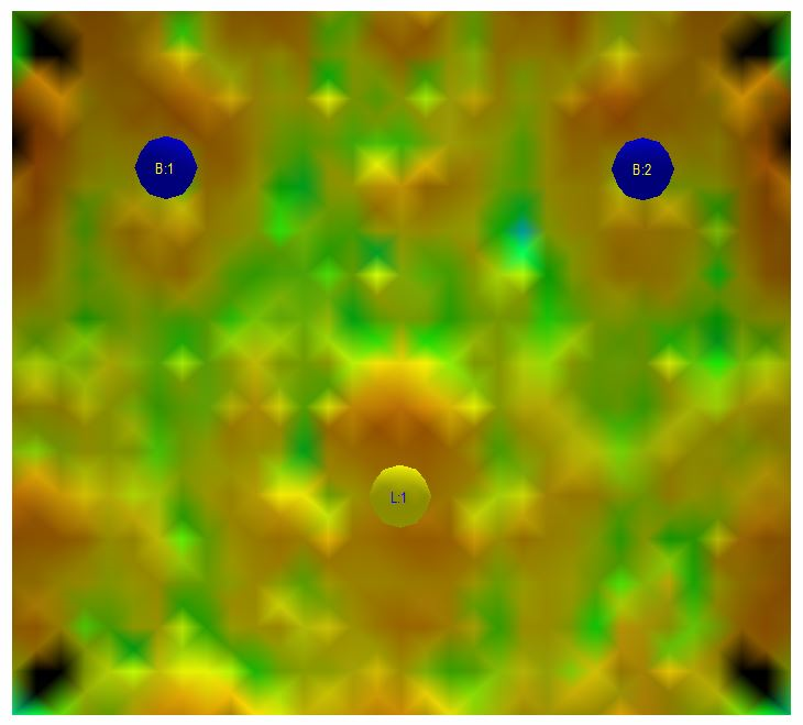
Fig 3.7: Steady state sound field at 217 Hz in the simulated room
Looking at the images it is evident that there is a dip at 74 Hz in the steady state sound pressure level at the listening position. There is a slight peak at 80 Hz as well as perhaps slightly more pronounced peaks at 160 Hz and 217 Hz. In different locations within the room there are various peaks and dips at the different frequencies. The peaks and dips are pretty well behaved since we took the trouble of acoustically treating the room the best we could. A measurement captured by a microphone located only at the listening position would show a response with the peaks and dips mentioned above. Unfortunately such a measurement would not correspond remotely with the sound perceived by a listener in the room. The common attempt for a workaround is then as mentioned earlier to use several measurement positions eventually capturing something approaching the power response in the room. The fundamental problem with power response measurements is however this; the steady state resonance sound field is built up over time and from measurements we know that it typically takes around 400 ms or longer for a loudspeaker to fully energize a room mode. In this context, room modes mean the resonances in the room that are caused by standing waves forming between the boundaries of the room, i.e. sound waves bouncing between walls, floor and ceiling. These room modes are present in the room regardless if there is a speaker or not in the room and are properties of the room itself. A build up time of 400 ms is a long time compared to most sounds generated by instruments and room mode effects are automatically without a conscious effort easy for us to suppress and distinguish as part of the room sound rather than the source we are listening to. As a consequence of our ability to suppress phenomena happening later in time it is not necessary or even preferable for a room correction system to try to deal with events that are delayed to such an extent. It’s actually quite easy to test this point, just talk to another person and walk together from one room to another. Is there any significant change to the voice? No, the voice remains the same but you can easily make out the different sounds reverberating or bouncing from the voice within the different rooms if you try to listen for it.
Our hearing has an impressive ability to resolve events in the time domain. The buildup of resonances in any material struck or note played on an instrument is used to determine the character of the material. Is it wood, metal, a trumpet or a violin? In fact, if the first millisecond or two is removed from an instrument’s initial sound it can actually become quite difficult to judge what type of instrument it is, there are many rather fun psychoacoustic experiments one can perform to experience this. Typically the first 5 ms are treated by our hearing as belonging to the initial or direct sound from a sound source. From about 5 ms to 15 ms it changes to a region where size of the sound source is judged. From about 25 ms the sound becomes discernible as a discrete echo. The mentioned boundaries in time are not fixed but rather flexible so they should not be considered as absolutes.
If we so easily without any apparent effort can resolve things that occur within a millisecond, does it then make sense to try to correct things that happens after several hundred milliseconds, probably not. One would rather think that it makes a strong case for getting the initial portion of the sound as accurate as possible, don’t you agree?
This is the predominant goal of the Böhmer Audio Room Compensation and why it’s operation and results are completely different from previous system.
Let’s have a look at the wave launch from the loudspeakers in the simulated room. The images below show how a short pressure wave propagates in the listening room. Think of it as the playback of a pressure wave from a very short thump. As usual, the two blue circles in the images are the loudspeakers and the yellow circle is at the listening position. The sound level is color coded; a darker color signifies a lower sound pressure level and a brighter more reddish a higher.
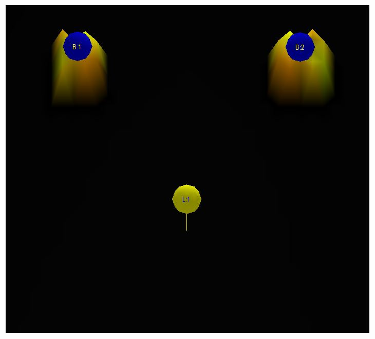
Fig 3.8: T0, the speakers have just now played the sounds, the room is still quiet
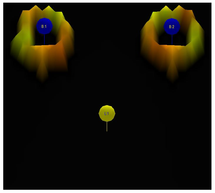
Fig 3.9: After 1.8 ms, the wave has just left the speakers. The wave travelling forward has a slightly higher sound pressure level than the one propagating back against the walls
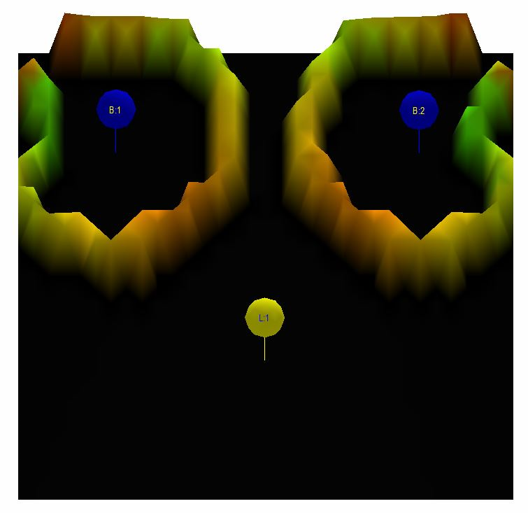
Fig 3.10: After 3.7 ms, the wave travelling back has just reached the back wall
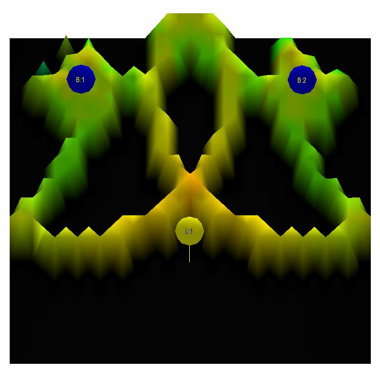
Fig 3.11: After 6.4 ms, the first wave front from the speakers is just about to arrive at the listening position. The second wave that initially moved back has bounced on the back and side walls and is now just in front of the loudspeakers
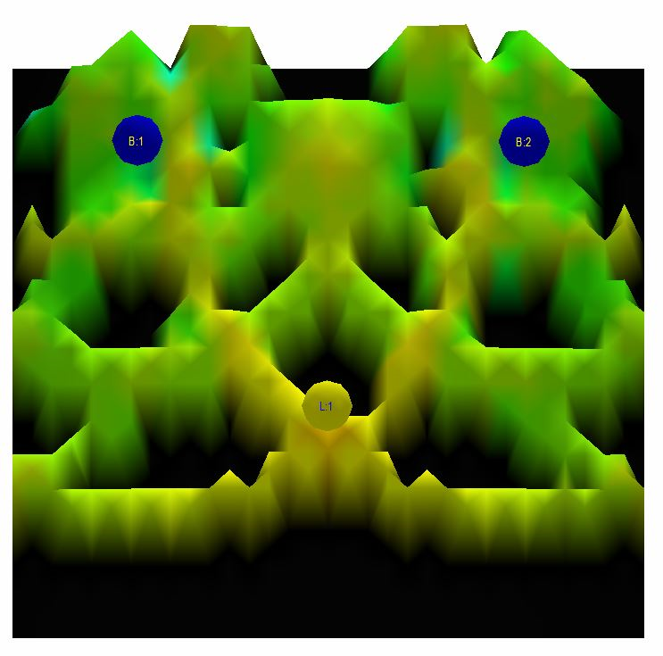
Fig 3.12: After 8.1 ms, the first wave front has arrived at the listening position. The second wave that initially moved back is only a few milliseconds behind
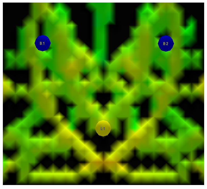
Fig 3.13: After 10.1 ms, the second wave front has arrived at the listening position. The first wave front is about to arrive at the back wall and bounce back
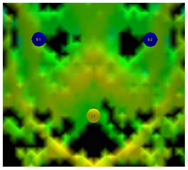
Fig 3.14: After 12.0 ms, the first wave front has bounced on the back wall and has arrived once again at the listening position. The second wave front is about to arrive at the back wall and bounce back
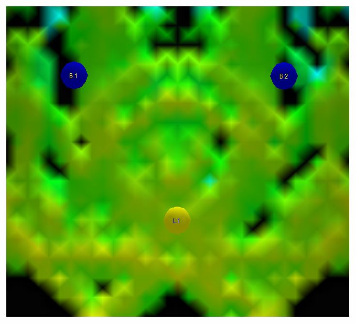
Fig 3.15: After 13.8 ms, the second wave front has bounced on the back wall and has arrived at the listening position again
It is now becoming more difficult to discern between the wave fronts in the room but the acoustic energy has just now, about 5 ms after the initial sound arrived at the listener, only come about half way back in the room. There is no chance that any room modes have begun to contribute. It is still only discrete wave fronts bouncing back and forth with complete silence in between (black areas). It will be at least another 20 ms or put another way 25 ms after the first sound arrived at the listening position before the energy is spread out in the room enough so it can begin to energize the room modes. Remember, after 25 ms our ears begin to be able to discern sounds as discrete echoes. Steady state room modes actually does not have that much to do with our perception of booming base within a room as one would easily think.
In summary, the initial sound pressure wave launched by a loudspeaker into a room is not influenced by any of the major dimensional room modes in the room during the first 25 ms. There are no peaks and dips in the frequency response in the room at this time because a standing wave pattern as shown in the steady state images earlier above hasn’t yet been established. This happens later in time. Our hearing easily and without effort resolves time domain phenomena within the single millisecond range. The usual power response doesn’t capture any of the crucial time domain information, only a steady state resonance field in the room that is slowly building up to full effect after about 400 ms or more.
Different results from different correction approaches
Hopefully the importance of measuring the correct phenomena in a room and the very high importance of the time domain has become a little bit clearer by now. Let’s consider the mathematics behind the correction method and have a closer look on how it influences the correction result.
Again, to improve visualization we go back to our simulated room and select the left speaker as our test object and simplify the setup a little only adding reflections from the front wall behind the speaker, left side wall, ceiling and floor.
The image below shows the steady state power frequency response of our left loudspeaker in the modified simulated room. The simulated loudspeaker is without any local frequency response deviations of its own only rolling of below about 25 Hz with a gentle response lift before and above 22 kHz again with a gentle lift. The local variations seen in the response is due to room modes and reflections from the front wall, left side wall, floor and ceiling. They look similar to what you’d expect to see in a normal time gated listening room frequency response measurement. All of the frequency response graphs shown below use a 200 ms time gating window to allow room modes to develop.
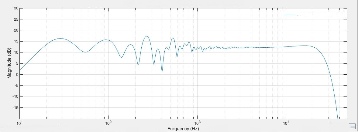
Fig 3.16: Left loudspeaker steady state power frequency response in modified listening room
The next image is a little more unusual, it is a wavelet response diagram. The time domain is shown top to bottom in the diagram, the frequency response left to right and the sound pressure level is color coded according to the color bar on the right. Ideally it should look like a straight Eiffel tower laying on its side. At the higher frequencies to the right the dark red ridge is very narrow because a period at those frequencies is short. To the left the ridge becomes progressively wider since the duration is longer at lower frequencies. One period at 10 kHz is only 100 µs, at 1 kHz it becomes 1ms and at 100 Hz it is 10 ms. This is seen as an elongation of the red ridge in the time domain. Any deviations of the dark red ridge from a straight line shows a time domain problem and any delayed energy shows up after the ridge as elongations of the duration of sound present at a particular frequency. The floor, celling and wall bounces are quite easy to spot in the diagram. One can also observe some time domain issues in the base region by the wavy appearance of the dark red ridge below approximately 200 Hz caused by the room. All of the wavelet diagrams below display the first 40 ms of the loudspeaker response. Remember, the modes just start to energize at about 25 ms and only reach full contribution after about 400 ms or more. At 40 ms there will be little contribution from them.
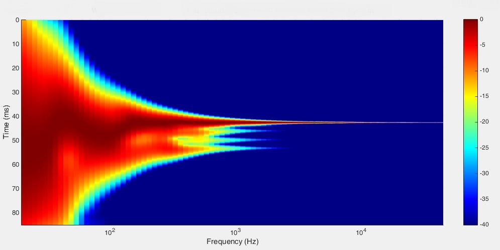
Fig 3.17: Left loudspeaker uncorrected wavelet response in modified listening room
If we now feed the captured power response measurement into an ordinary power response based correction system that only looks on the problem in the frequency domain it comes up with the correction solution shown in the image below.
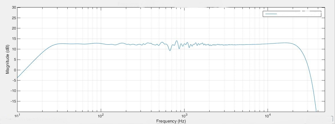
Fig 3.18: Left loudspeaker power response room correction result
The frequency response with the power response correction looks good doesn’t it? Almost all of the nasty wiggles in the frequency response are gone and the loudspeaker’s own response reemerges. This must sound good don’t you think? Well, maybe not as well se shortly.
Below is the steady state power frequency response created by the Böhmer Audio Room Compensation System under the same conditions. It doesn’t look nearly as good; it has removed some of the dips and peaks to some extent but not as much as the power response system earlier did. How can it then be superior?
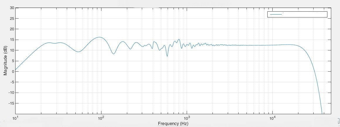
Fig 3.19: Left loudspeaker Böhmer Audio Room Compensation result
The explanation is that the Böhmer Audio Room Compensation looks on the response primarily in the time domain and not so much in the frequency domain. The image below shows the wavelet response after the Böhmer Audio Room Compensation. There is a remarkable improvement with the time domain now looking almost perfect up to above approximately 400 Hz where some energy from the reflections still remain. These frequencies are actually above the range where the correction predominantly operates. It is designed that way because it is difficult to obtain predictably good results at higher frequencies. What the image also shows is that during at least the first 40 ms, the response from the loudspeaker in the room is more or less perfect without any aberrations. This then changes gradually during 200 ms to the frequency response graph show above. Instead of focusing the correction on the frequency response of the loudspeaker and room at an arbitrary point later in time the Böhmer Audio Room Compensation makes it perfect in the beginning when it really counts. What happens at 100ms, 200 ms or 400 ms, who cares, no one is listening anyway…
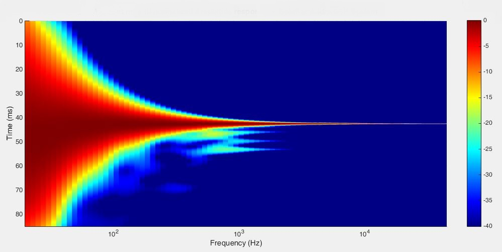
Fig 3.20: Left loudspeaker Böhmer Audio Room Compensation result
So the final question, how does the power response correction look like in the time domain? The image below show the first 40 ms seconds of it.
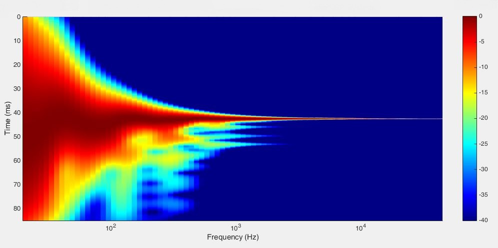
Fig 3.21: Left loudspeaker power response room correction result
Well, obviously that doesn’t look all that good. If we compare with the uncorrected loudspeaker it has managed to clean up some of the reflected energy but unfortunately it creates a lot of new energy long after the initial ridge lower down in the diagram that is not present in the uncorrected measurement. Such high energy levels so late in time is not a good thing and the result will audibly most likely be perceived as a little bit if a mixed bag. Some things improve while others do not. The late energy often gives an artificial flavour to the sound and the improvement of perceived timing would be uncertain.
The frequency response does look very good though but the results earlier in time are unpredictable since information about the behaviour is not present in the measurement and consequently can’t be corrected for by the algorithms. The addition of severely delayed energy is a common outcome of the process. Traditional room correction systems are often accused of producing unpredictable and sometimes worse results than an uncorrected system and this is the reason.
What of the rest of the room, not just the listening position
One problem with earlier room correction systems has been that the perceived sound quality at other locations in the room than the listening position is sometimes worse than from an uncorrected speaker. The root of the problem is that they fail to address the fundamental issue of loudspeaker energy launch into the room. Just look on the wavelet diagram above from the power response correction, the launch is anything but even. If the loudspeaker initially launches an uneven amount of energy at different frequencies into the room the sound energy field in the room will be uneven. If the loudspeaker launches and even amount of energy into the room, as is done by the Böhmer Audio Room Compensation, the sound field will be even.
This is easily verified by walking around in a room with a loudspeaker system corrected by the Böhmer Audio Room Compensation comparing it with an uncorrected system and with a power response corrected system. The Böhmer Audio Room Compensated system will sound controlled, transient phenomena are well defined and boominess is absent anywhere in the room, the uncorrected system will be perceived as slightly soft, lacking articulation and having a rubber bandisch quality to the sound with some booming and the power response corrected system is, well you might have guessed, a bit unpredictable.
This is not at all a subtle effect, once you’ve heard it a couple of times you will be able to spot a Böhmer Audio Room Compensated system instantly when you just enter a listening room. No need to be even close to the listening area.